Energy Project Economics: LCOE Modeling Framework

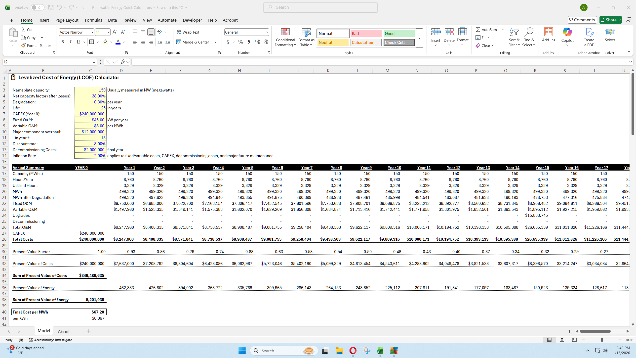
This Excel model is a practical, top-down tool for estimating the Levelized Cost of Energy (LCOE)—the average cost to generate electricity over the full life of a power project, expressed in today’s dollars. It’s built to help you answer one core question:

“If I build and run this power plant, what is the lifetime cost per unit of electricity produced?”

Because it standardizes the result as a cost per MWh, the model is useful for comparing very different technologies—solar, wind, nuclear, gas, or others—on a consistent basis.
What the Model Is Designed to Do

At a high level, the model converts a complex, multi-year project into a single comparable metric by:

1. Forecasting energy production year-by-year across the project life
   
   

2. Forecasting costs across the same timeline (upfront, recurring, and one-time)
   
   

3. Converting both of those streams into present value using a discount rate
   
   

4. Dividing the total discounted costs by the total discounted energy to produce LCOE
   
   

That structure makes the model easy to use in early-stage evaluation, investment screening, and scenario analysis—without requiring a full project finance model.
The Core Logic in Plain English

The model treats a power project like two streams running in parallel over time:
1) Energy Stream

The plant produces electricity each year. The model estimates annual production using a few key drivers like:

• nameplate capacity
  
  

• capacity factor
  
  

• degradation over time
  
  

• length of project life
  
  

Because the plant typically produces less energy over time (due to wear, soiling, equipment aging, etc.), the model includes a degradation rate so production trends downward in a realistic way.
2) Cost Stream

Costs show up in different shapes:

• Upfront CAPEX (initial build cost)
  
  

• Ongoing operating costs (fixed and variable O&M)
  
  

• Scheduled major replacements or overhauls (one-time, year-specific events)
  
  

• End-of-life costs (decommissioning)
  
  

Future costs can be escalated using an inflation rate, so you can represent rising nominal expenses over time.
Why Discounting Matters

The model uses a discount rate to express future costs and future energy in present-value terms. This is important because:

• A dollar spent 15 years from now is not the same as a dollar spent today
  
  

• A MWh produced 15 years from now is not the same as a MWh produced today (in economic value terms)
  
  

By discounting both costs and production, LCOE becomes a fair “apples-to-apples” measure of lifetime economics.
Outputs You Get From the Model

The main output is the project’s:

• Final cost per MWh (primary metric)
  
  

• Final cost per kWh (same metric in a different unit)
  
  

To keep the result transparent, the model also outputs:

• Present Value of Total Costs
  
  

• Present Value of Total Energy Produced
  
  

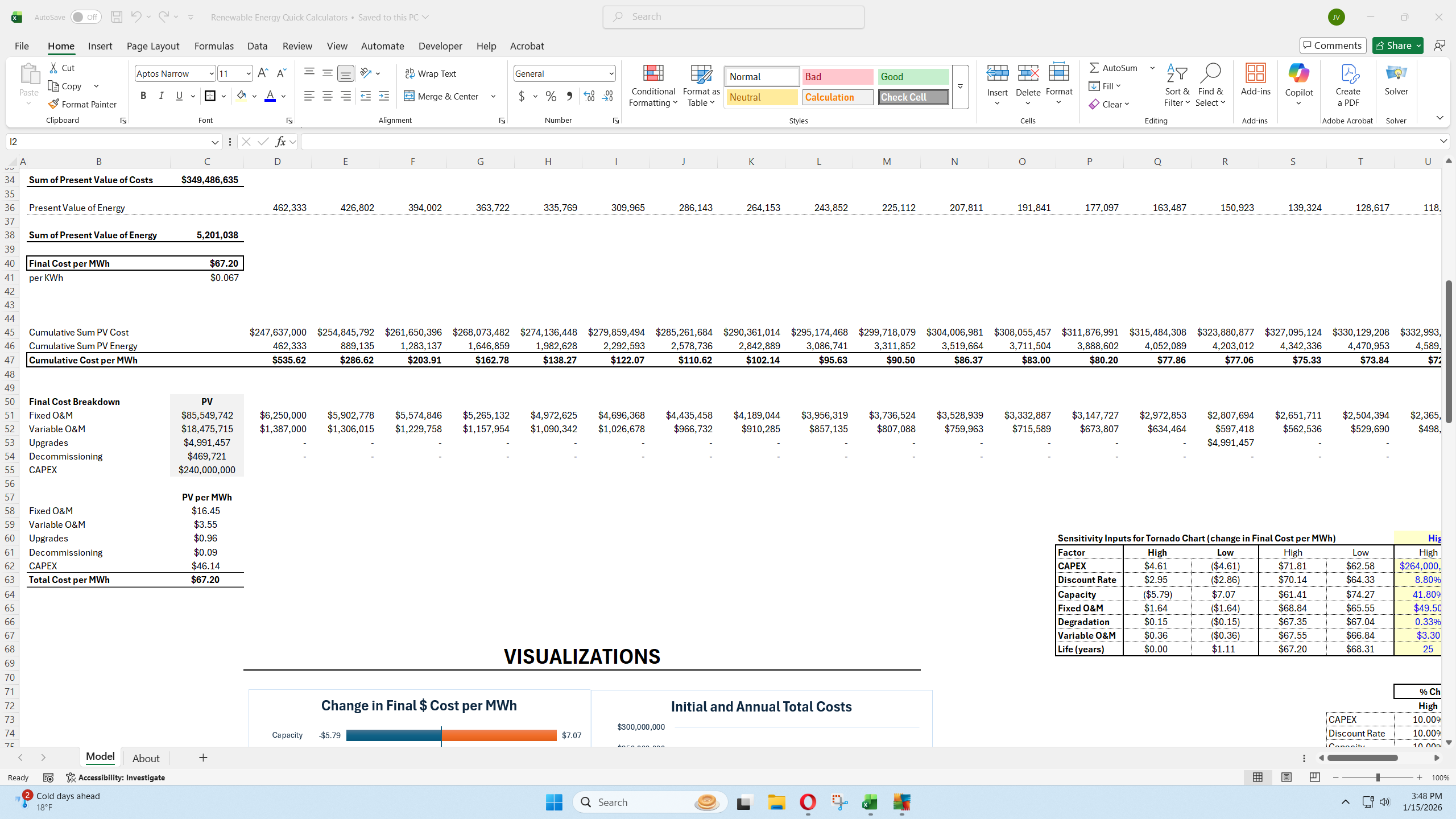
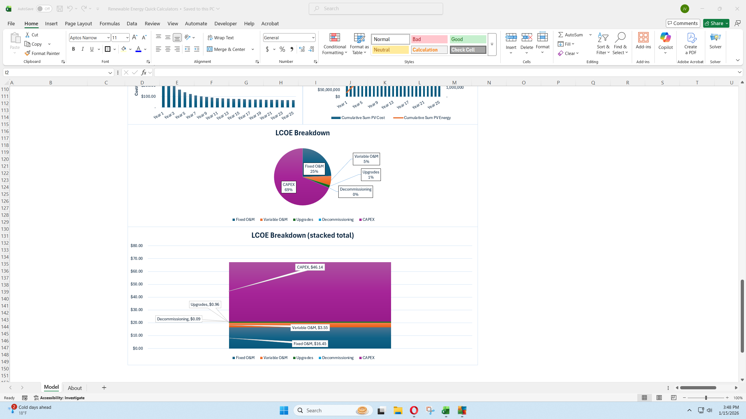
• A cost breakdown, so you can see which categories drive the result
  
  

This matters because two projects can have the same LCOE for totally different reasons (high capex vs high opex, expensive overhaul vs low capacity factor, etc.).
What Makes This Model Easy to Use

The model is designed for speed and portability:

• Single-tab build: inputs, calculations, and visuals in one place
  
  

• Clear input/formula formatting: easy to see what you can change safely
  
  

• Scenario-friendly: change assumptions and instantly see impacts
  
  

• Up to 25-year horizon: enough to cover most utility-scale assets and many commercial/industrial projects
  
  

It’s intentionally structured so you can drop it into an existing workbook or use it as a standalone evaluator.
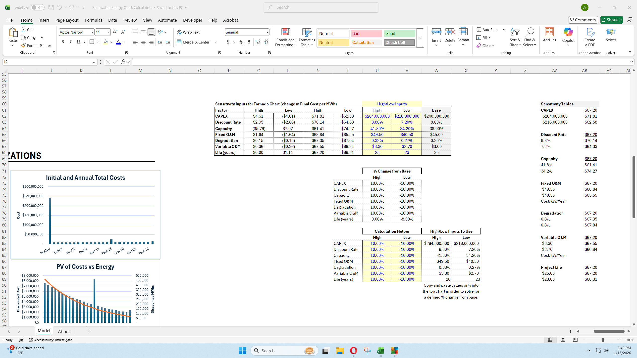
High-Level Sensitivity and the Tornado Chart

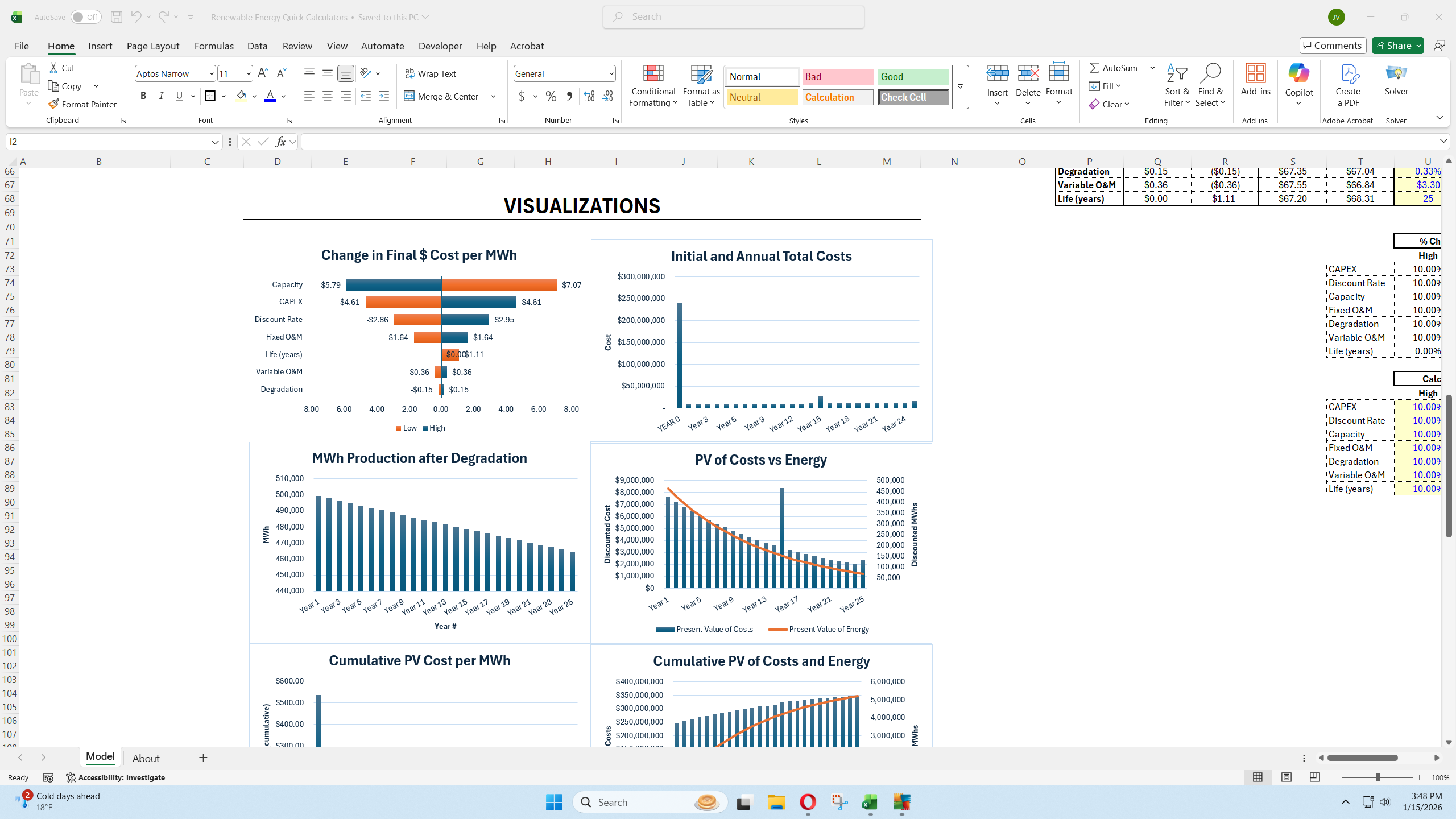
One of the most useful “executive level” features is the tornado sensitivity chart, which summarizes how sensitive the LCOE result is to key assumptions.

At a high level, it:

• applies a +/- change to each major driver (one at a time)
  
  

• calculates the resulting change in LCOE
  
  

• ranks the drivers by impact so you immediately know what matters most
  
  

This is particularly valuable for:

• prioritizing diligence (what assumptions deserve the most scrutiny)
  
  

• explaining results to stakeholders
  
  

• comparing projects where the uncertainty profile differs
  
  

The chart’s ranking updates automatically, so you don’t have to manually re-sort anything as inputs change.
When This Model Is Most Useful

This is a high-level economic lens, so it’s best used for:

• early-stage feasibility checks
  
  

• comparing technology options on consistent terms
  
  

• “what-if” scenario modeling (capex up/down, capacity factor changes, O&M assumptions, discount rate shifts)
  
  

• communicating project economics in a clean, standardized way
  
  

It’s also a good companion to (not a replacement for) more detailed project finance models—because it is focused on unit cost of energy, not full cash waterfall, tax equity structuring, or revenue stack modeling.