How to Apply The Central Limit Theorem

The reason for this is the unmatched practical application of the theorem.


Ok.


Let’s get started then.


Imagine that you are given a data set. Its distribution does not matter. It could be Normal, Uniform, Binomial or completely random.


The first thing you want to do is start taking out subsets from the data set, or as statisticians call it – you start sampling it. This would allow you to gain a better idea of how the entire data set is made, right?


Ok.


Once you have taken a sufficient number of samples and then calculated the mean of each sample, we’ll be able to apply the central limit theorem.


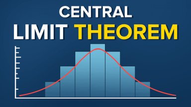
No matter the distribution of the entire data set, Binomial, Uniform or another one, the means of the samples you took from the entire data set will approximate a normal distribution.


The more samples you extract and the bigger they are, the closer to a normal distribution the sample means will be. Moreover, their distribution will have the same mean as the original data set and an n times smaller variance, where n is the size of the samples you took from the data set.


Let’s confirm the theorem with an example. We have prepared 960 random numbers from 1 to 1000. This is their frequency distribution so you are sure that they are randomly picked. The mean of this data set is 489 and its variance is 82,805.


Let’s extract 30 random samples out of the data set, each consisting of 25 numbers. Remember when we said that the sample should be sufficiently large? A common rule of thumb is that the sample should be bigger than 25 observations. The bigger the sample size, the better results you’ll get.


So, we have our samples. Now we are going to calculate their means and plot them once again.


Ok. Excellent!


It looks approximately normally distributed, doesn’t it! Let’s check if the other part of the theorem was right. The mean of our newly acquired data set is 492, while its variance – 3171.
Did we expect these numbers? We anticipated a mean of 489 and a variance of 82,805 divided by 25, so around 3,312.


Well, when dealing with such big numbers we almost got the mean right and the variance was not that far off either. In the next few lectures you will learn how to statistically confirm whether such small differences are close enough to the actual result we expect to obtain.


Spoiler alert – they are J , and we’ll show you why!


So, we have learned the main idea behind the central limit theorem.


The key take-away from this lesson is that as the number of samples taken tends towards infinity, the distribution of the means starts approximating a normal distribution. Imagine their power if your dataset was made up of millions of values and you could afford to sample just a tiny bit of them! We can be assuming normally distributed data almost all the time. And that’s extremely helpful.