Salary Tax Calculator using Microsoft Excel's LAMBDA & LET Functions for Financial Year 2026-2027 (Tax Year 2027)

Description
Turn a formula into reusable function via LAMBDA
LAMBDA lets us write a custom function once, give it a name (via the Name Manager), and call it anywhere. Just like SUM or VLOOKUP, except we defined it. The pattern LAMBDA(parameter1, parameter2, ..., formula_using_the_parameters) is saved under a name.


The Calculate name does exactly this.
Calculate = LAMBDA(TaxableIncome, TaxRate, MonthlySalary, LET(a, SORT(VSTACK(MonthlySalary, DROP(TaxableIncome, 1))), SUM((a - TaxableIncome) * TaxRate)))


It takes three inputs; the slab thresholds, the matching rates, and one salary; and returns the tax owed. Once defined, =Calculate(Slabs[Taxable Income], Slabs[Tax Rate], 1067328) behaves exactly like a built-in function call.


What Calculate is actually doing
This is the part worth walking through, because "insert the salary into the sorted list of thresholds" is a clever but non-obvious trick:


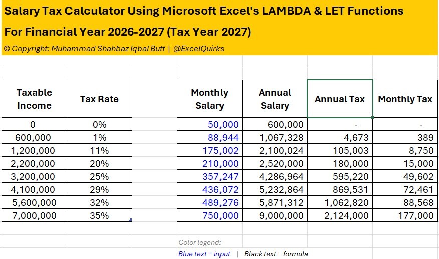
With a real row from our sheet where monthly salary 88,944 → annual salary 1,067,328:
Drop lowest slab: {0, 600k, 1.2M, 2.2M, 3.2M, 4.1M, 5.6M, 7M} → drop the 0 → {600k, 1.2M, 2.2M, 3.2M, 4.1M, 5.6M, 7M}
Add annual salary: stack 1,067,328 on top → {1,067,328, 600k, 1.2M, 2.2M, 3.2M, 4.1M, 5.6M, 7M}
Sort ascending: {600k, 1,067,328, 1.2M, 2.2M, 3.2M, 4.1M, 5.6M, 7M}. The salary now sits between the 600k and 1.2M thresholds, exactly where it belongs
Subtract & weight: each sorted value minus the original slab threshold, times that slab's rate → for the 600k slab: (600,000 − 0) × 0% = 0; for the 1.2M slab: (1,067,328 − 600,000) × 1% = 4,673.28; every slab above the salary subtracts to zero, so it contributes nothing
Sum: 0 + 4,673.28 + 0 + 0 + 0 + 0 + 0 + 0 = 4,673 (after rounding) thus matching G8 in our sheet exactly


The trick is that sorting always inserts the salary right where it belongs, so only the brackets below it produce a positive number; every step above collapses to zero automatically. That's what makes it a "one-formula" tax calculator instead of a chain of IFs.


How they combine in our sheet

G7 doesn't call Calculate once; it uses BYROW(ANCHORARRAY(F7), LAMBDA(Salary, Calculate(...))) to run this whole five-step process once per row, automatically, for every salary in the spill range. That's LAMBDA (a reusable function) and LET/dynamic arrays (naming and reshaping data) working together: one calculates the number, the other applies it row by row.