Originally published: 18/07/2022 12:12
Publication number: ELQ-87695-1
View all versions & Certificate
Publication number: ELQ-87695-1
View all versions & Certificate

Waste to Energy / Biogas Project Finance Model
Waste to Energy Biogas Project Finance Model presents the case of an investment in the construction of a biomass processing plant and the sale of the energy.
waste to energybiogasproject financebiomassthree statementsscenariosbreak evenkpisvaluationfinancial model
Description
Waste to Energy Biogas Project Finance Model presents the business case of an investment in the construction of a biomass processing plant and the sale of the energy generated from it, as well as by products from the process. The model generates the three financial statements as well as the cash flows and calculates the relevant metrics (cash on cash, Internal Rate of Return, payback period, Net Present Value, Debt Service Coverage Ratio, Loan Life Coverage Ratio, Weighted Average Loan Life). The financing options for the project include 2 senior tranches, 1 junior tranche, as well as a working capital facility and of course equity funding from investors.
The model generates:
1) Three financial statements (profit & loss, balance sheet and cash flow)
2) Valuation using free cash flows
3) Returns and KPIs
4) Breakeven analysis
5) Margins, ratios, and feasibility metrics
6) Three scenarios to stress test the plan in the "Scenarios" tab
7) Executive Summary tab which aggregates the most important metrics of the model.
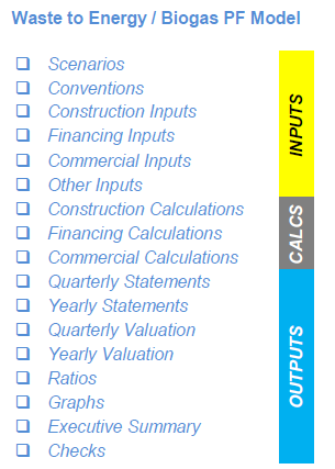
So, a quick overview of the model, in the contents tab you can see the structure of the model and by clicking on any of the headlines to be redirected to the relevant worksheet.
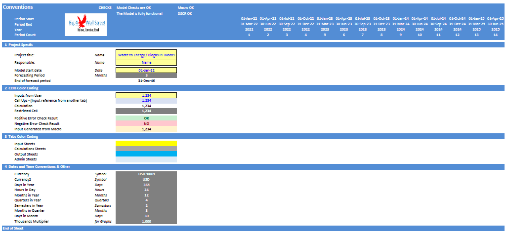
On the Conventions tab you are able to feed the general information for the model such as: model name, responsible, timeline of the model and date and currency conventions. Additionally there is a description of the color coding of the model in the same tab. Inputs are always depicted with a yellow fill and blue letters, call ups (that is direct links from other cells) are filled in light blue with blue letters while calculations are depicted with white fill and black characters. There is also a color coding for the various tabs of the model. Yellow tabs are mostly assumptions tabs, grey tabs are calculations tabs, blue tabs are outputs tabs (that is effectively results or graphs) and finally light blue tabs are admin tabs (for example: the cover page, contents and checks).
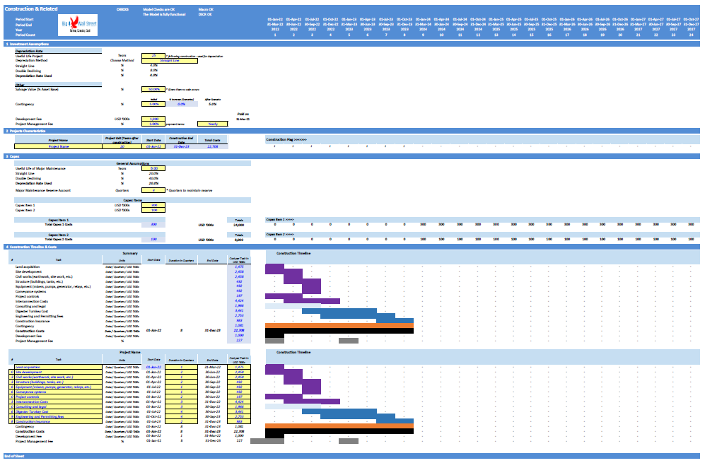
The Construction Tab contains the main investment assumptions such as useful life of the project, depreciation method (the user can choose between straight line and double declining), the salvage value at the exit of the investment, the contingency percentage which will increase the baseline construction costs. Furthermore the user sets in this tab the development fee (which is paid when the debt is drawn), the project management fee as a percentage construction costs (this fee can be paid on an annual or quarterly basis). Next the user sets the project name, the project exit (in years after the construction), and the construction start date. Additionally it is possible for the user to set the capex items on a quarterly items, the needed capex reserve account in terms of quarters and their corresponding useful life. Finally the user can set the timeline of the construction for each task, and their duration in quarters, as well as the cost per task. All the above are calculated and allocated in the Construction Calculations tab.
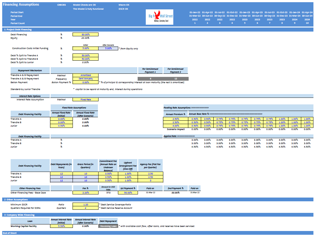
Moving to the Financing Tab, the user sets the percentage of debt financing, the construction costs initial funding from equity, and the debt split between senior tranches (A and B), and junior tranches. The user selects the repayment method for the senior tranches (amortized or debt sculpting), as well as the repayment frequency (semi annual or quarterly), and the balloon payment if any (up to 100%). The user then selects between fixed and variable interest rates, and adjusts the corresponding rates for each of these calculations methods, and for each tranche separately. The user also sets the debt repayment in years, the grace period, as well as the other financing fees such as commitment fees, upfront fess, agency fees and other financing fees. Finally the user sets the interest rate for the working capital facility. All the above assumptions are used for the calculations performed in the Financing Calculations tab.
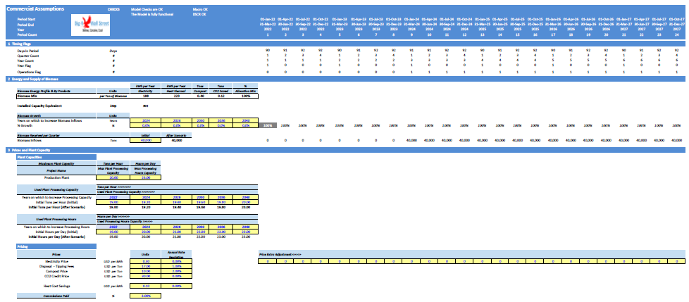
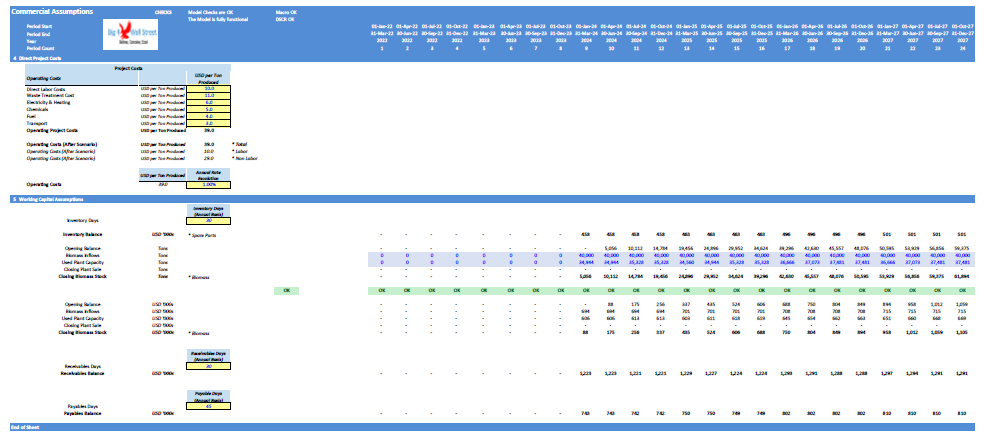
In the Commercial Tab, the user can set the energy profile for each biomass type such as energy production, heat production, allocation mix, and their by products such as compost and C O 2 saved. Afterwards the user sets the biomass inflows tons and growth rate per selected year. Then the user sets the maximum plant capacity in tons per hour, and hours per day, as well as the planned tons per hour, and hours per day, for each selected year. Continuing the user set the prices and growth rates for the various products sold such as electricity price, tipping fees, compost price, and C O 2 credit price, as well as the opportunity cost of heat savings. The remaining items consist of direct project costs per ton produced (such as direct labor, waste treatment, electricity and heating, chemicals, fuel, and transport), and their growth rate. Finally the working capital assumptions for inventory, receivables and payables days. All the above assumptions are used for the calculations performed in the Commercial Calculations tab.
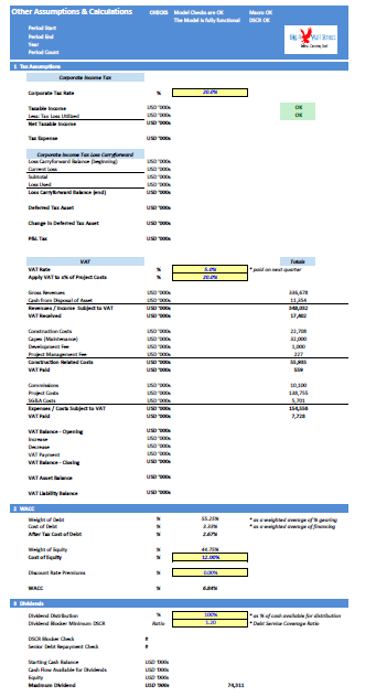
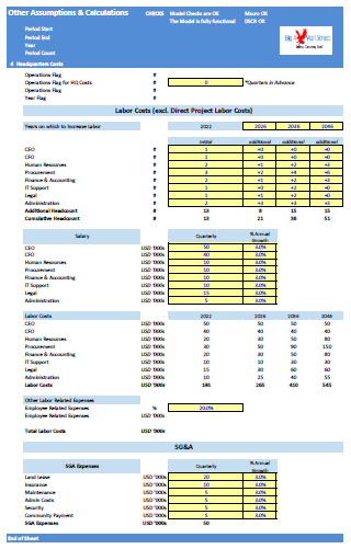
The Other Tab contains tax assumptions, discount rate assumptions, dividends assumptions, and finally headquarters' labor and sales and general administrative costs. The labor assumptions include headcount and salary for each position as well as employment related expenses. The calculations are performed in the same tab.
After finalizing your assumptions press the "Calculate Financing" button to update the Outputs tabs.
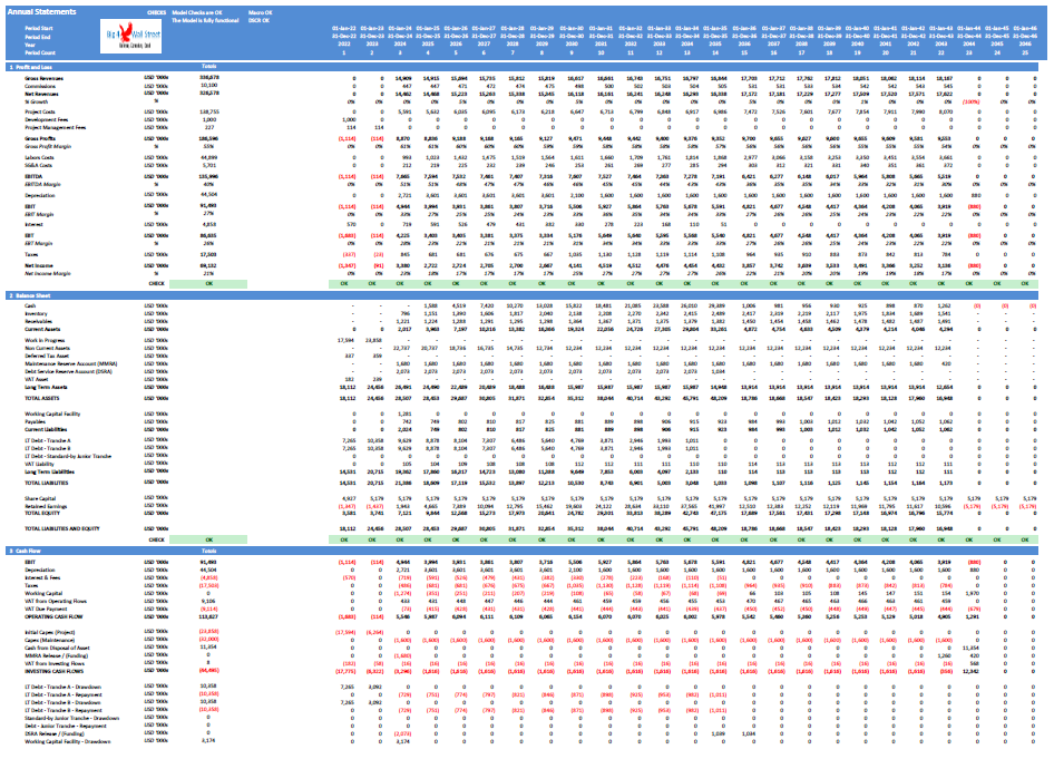
Financial Statement Tabs: everything is aggregated here into the relevant statements: profit and loss, balance sheet and cash flow, both on a quarterly and annual basis.
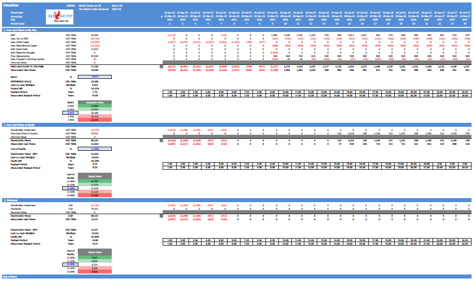
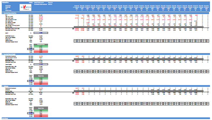
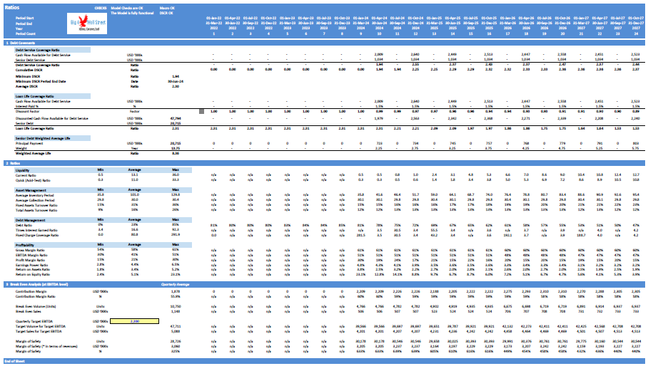
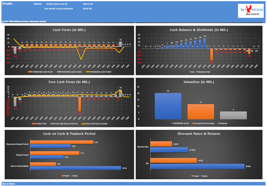
The Valuation is performed both on a quarterly and annual basis, by using the free cash flows to the firm, free cash flows to equity, dividends discount method. In this tab are calculated the Enterprise Value, Net Present Value, the Cash on Cash Multiple, the Internal Rate of Return, and Payback Period. In the next tab, the Ratio tab, the model calculates the debt service coverage and loan life coverage ratio, as well as the senior debt weighted average life. Afterwards a series of ratios are calculated, and a break even analysis is performed at an EBITDA level.
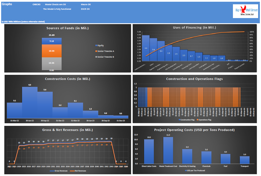
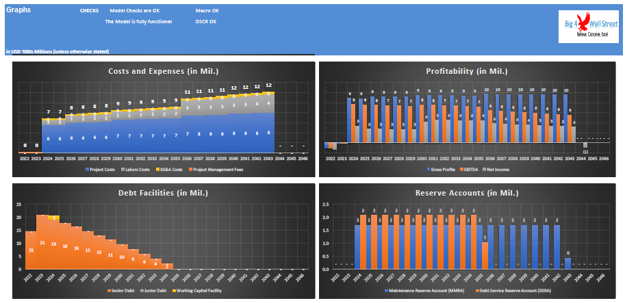
Graphs Tab: Various graphs present the investment & operating costs as well as the energy generation potential. Then multiple charts present the performance of the project from revenues to bottom line along with debt, assets, working capital and cash flows which results in a valuation on a project basis as well as on an equity basis together with the internal rate of return of the project and payback period metrics.
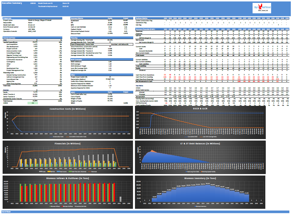
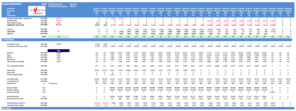
Executive Summary: the summary page is updated with the main output metrics of the model such as Internal Rate of Return, Shareholder Value, Cash on Cash Multiple, Sources and Uses, Biomass Flows and Inventory, Debt Service Coverage Ratio, Loan Life Coverage Ratio, and other financing assumptions.
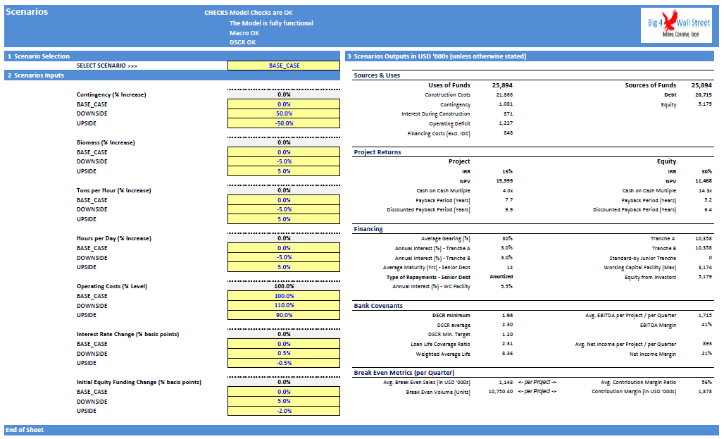
The user can also set three different scenarios: Base Case, Downside and Upside. The user can set for each scenario the percentage increase of the contingency, the biomass, the tons per hour, the hours per day, the opeating costs level, the interest rate basis points change, and the initial equity funding basis points change. After the user sets the assumptions and selects the scenarios, the user needs to press the "Calculate FInancing" button. On the right side of the tab, the user can see the updated major metrics of the model.
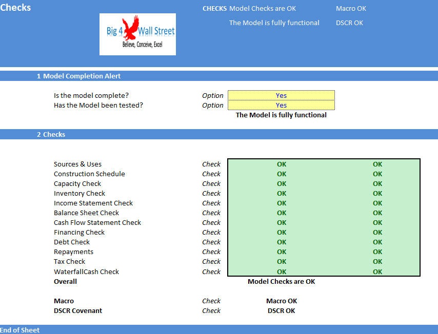
Checks: A dedicated worksheet that makes sure that everything is working as it should!
Waste to Energy Biogas Project Finance Model presents the business case of an investment in the construction of a biomass processing plant and the sale of the energy generated from it, as well as by products from the process. The model generates the three financial statements as well as the cash flows and calculates the relevant metrics (cash on cash, Internal Rate of Return, payback period, Net Present Value, Debt Service Coverage Ratio, Loan Life Coverage Ratio, Weighted Average Loan Life). The financing options for the project include 2 senior tranches, 1 junior tranche, as well as a working capital facility and of course equity funding from investors.
The model generates:
1) Three financial statements (profit & loss, balance sheet and cash flow)
2) Valuation using free cash flows
3) Returns and KPIs
4) Breakeven analysis
5) Margins, ratios, and feasibility metrics
6) Three scenarios to stress test the plan in the "Scenarios" tab
7) Executive Summary tab which aggregates the most important metrics of the model.
So, a quick overview of the model, in the contents tab you can see the structure of the model and by clicking on any of the headlines to be redirected to the relevant worksheet.
On the Conventions tab you are able to feed the general information for the model such as: model name, responsible, timeline of the model and date and currency conventions. Additionally there is a description of the color coding of the model in the same tab. Inputs are always depicted with a yellow fill and blue letters, call ups (that is direct links from other cells) are filled in light blue with blue letters while calculations are depicted with white fill and black characters. There is also a color coding for the various tabs of the model. Yellow tabs are mostly assumptions tabs, grey tabs are calculations tabs, blue tabs are outputs tabs (that is effectively results or graphs) and finally light blue tabs are admin tabs (for example: the cover page, contents and checks).
The Construction Tab contains the main investment assumptions such as useful life of the project, depreciation method (the user can choose between straight line and double declining), the salvage value at the exit of the investment, the contingency percentage which will increase the baseline construction costs. Furthermore the user sets in this tab the development fee (which is paid when the debt is drawn), the project management fee as a percentage construction costs (this fee can be paid on an annual or quarterly basis). Next the user sets the project name, the project exit (in years after the construction), and the construction start date. Additionally it is possible for the user to set the capex items on a quarterly items, the needed capex reserve account in terms of quarters and their corresponding useful life. Finally the user can set the timeline of the construction for each task, and their duration in quarters, as well as the cost per task. All the above are calculated and allocated in the Construction Calculations tab.
Moving to the Financing Tab, the user sets the percentage of debt financing, the construction costs initial funding from equity, and the debt split between senior tranches (A and B), and junior tranches. The user selects the repayment method for the senior tranches (amortized or debt sculpting), as well as the repayment frequency (semi annual or quarterly), and the balloon payment if any (up to 100%). The user then selects between fixed and variable interest rates, and adjusts the corresponding rates for each of these calculations methods, and for each tranche separately. The user also sets the debt repayment in years, the grace period, as well as the other financing fees such as commitment fees, upfront fess, agency fees and other financing fees. Finally the user sets the interest rate for the working capital facility. All the above assumptions are used for the calculations performed in the Financing Calculations tab.
In the Commercial Tab, the user can set the energy profile for each biomass type such as energy production, heat production, allocation mix, and their by products such as compost and C O 2 saved. Afterwards the user sets the biomass inflows tons and growth rate per selected year. Then the user sets the maximum plant capacity in tons per hour, and hours per day, as well as the planned tons per hour, and hours per day, for each selected year. Continuing the user set the prices and growth rates for the various products sold such as electricity price, tipping fees, compost price, and C O 2 credit price, as well as the opportunity cost of heat savings. The remaining items consist of direct project costs per ton produced (such as direct labor, waste treatment, electricity and heating, chemicals, fuel, and transport), and their growth rate. Finally the working capital assumptions for inventory, receivables and payables days. All the above assumptions are used for the calculations performed in the Commercial Calculations tab.
The Other Tab contains tax assumptions, discount rate assumptions, dividends assumptions, and finally headquarters' labor and sales and general administrative costs. The labor assumptions include headcount and salary for each position as well as employment related expenses. The calculations are performed in the same tab.
After finalizing your assumptions press the "Calculate Financing" button to update the Outputs tabs.
Financial Statement Tabs: everything is aggregated here into the relevant statements: profit and loss, balance sheet and cash flow, both on a quarterly and annual basis.
The Valuation is performed both on a quarterly and annual basis, by using the free cash flows to the firm, free cash flows to equity, dividends discount method. In this tab are calculated the Enterprise Value, Net Present Value, the Cash on Cash Multiple, the Internal Rate of Return, and Payback Period. In the next tab, the Ratio tab, the model calculates the debt service coverage and loan life coverage ratio, as well as the senior debt weighted average life. Afterwards a series of ratios are calculated, and a break even analysis is performed at an EBITDA level.
Graphs Tab: Various graphs present the investment & operating costs as well as the energy generation potential. Then multiple charts present the performance of the project from revenues to bottom line along with debt, assets, working capital and cash flows which results in a valuation on a project basis as well as on an equity basis together with the internal rate of return of the project and payback period metrics.
Executive Summary: the summary page is updated with the main output metrics of the model such as Internal Rate of Return, Shareholder Value, Cash on Cash Multiple, Sources and Uses, Biomass Flows and Inventory, Debt Service Coverage Ratio, Loan Life Coverage Ratio, and other financing assumptions.
The user can also set three different scenarios: Base Case, Downside and Upside. The user can set for each scenario the percentage increase of the contingency, the biomass, the tons per hour, the hours per day, the opeating costs level, the interest rate basis points change, and the initial equity funding basis points change. After the user sets the assumptions and selects the scenarios, the user needs to press the "Calculate FInancing" button. On the right side of the tab, the user can see the updated major metrics of the model.
Checks: A dedicated worksheet that makes sure that everything is working as it should!
This Best Practice includes
1 Excel and 1 PDF