
Publication number: ELQ-55943-1
View all versions & Certificate

Intermittent Demand Forecasting for Spare Parts — SES, Croston, SBA, SBJ & Auto-Selection Excel Model
Academically and professionally grounded spare parts forecasting. From demand signals to order quantity.
 by Prince Ntow
Supply Chain Management Professional with extensive experience in Logistics, Inventory Management . Data driven problem solver.Follow
Further information
1. Correct the most common forecasting error in spare parts management
Demonstrate why applying standard moving averages or simple exponential smoothing to intermittent demand series produces systematically misleading forecasts, and replace that approach with statistically validated alternatives.
2. Automate demand classification at the SKU level
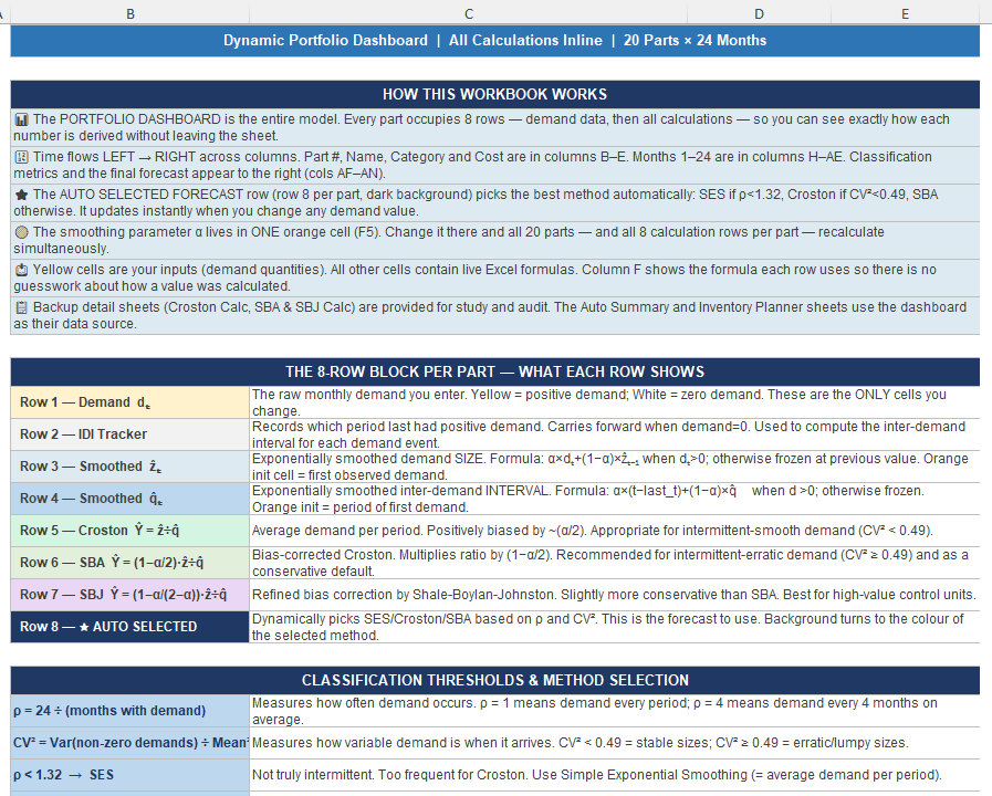
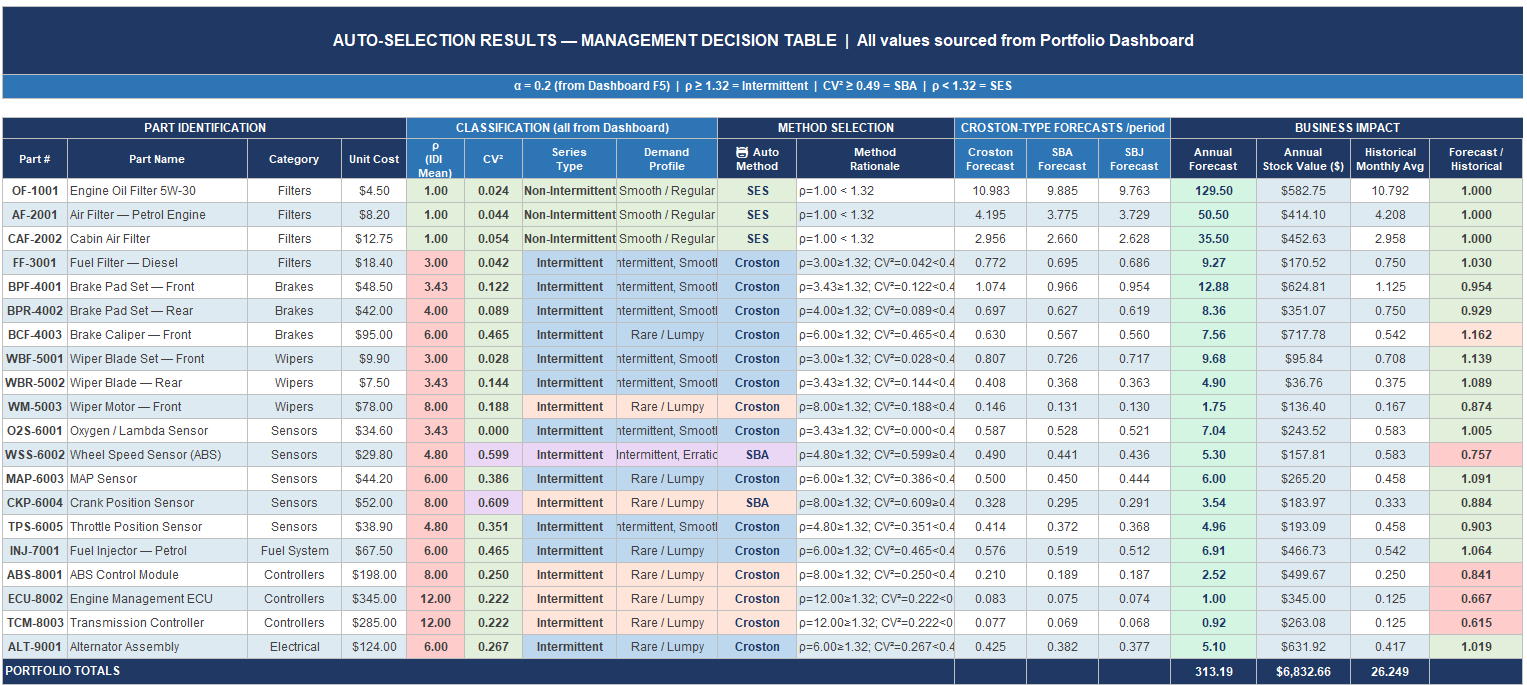
Equip practitioners with a live, formula-driven classification engine that computes ρ (inter-demand interval mean) and CV² (demand size variability) for every SKU and automatically routes each one to the appropriate forecasting method: SES, Croston, or SBA, without manual intervention.
3. Make the forecasting mechanics fully transparent
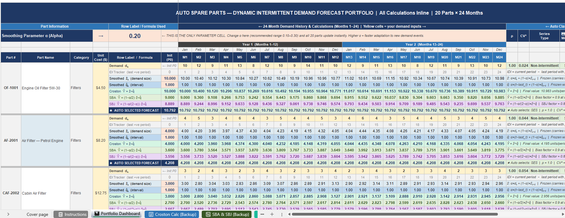
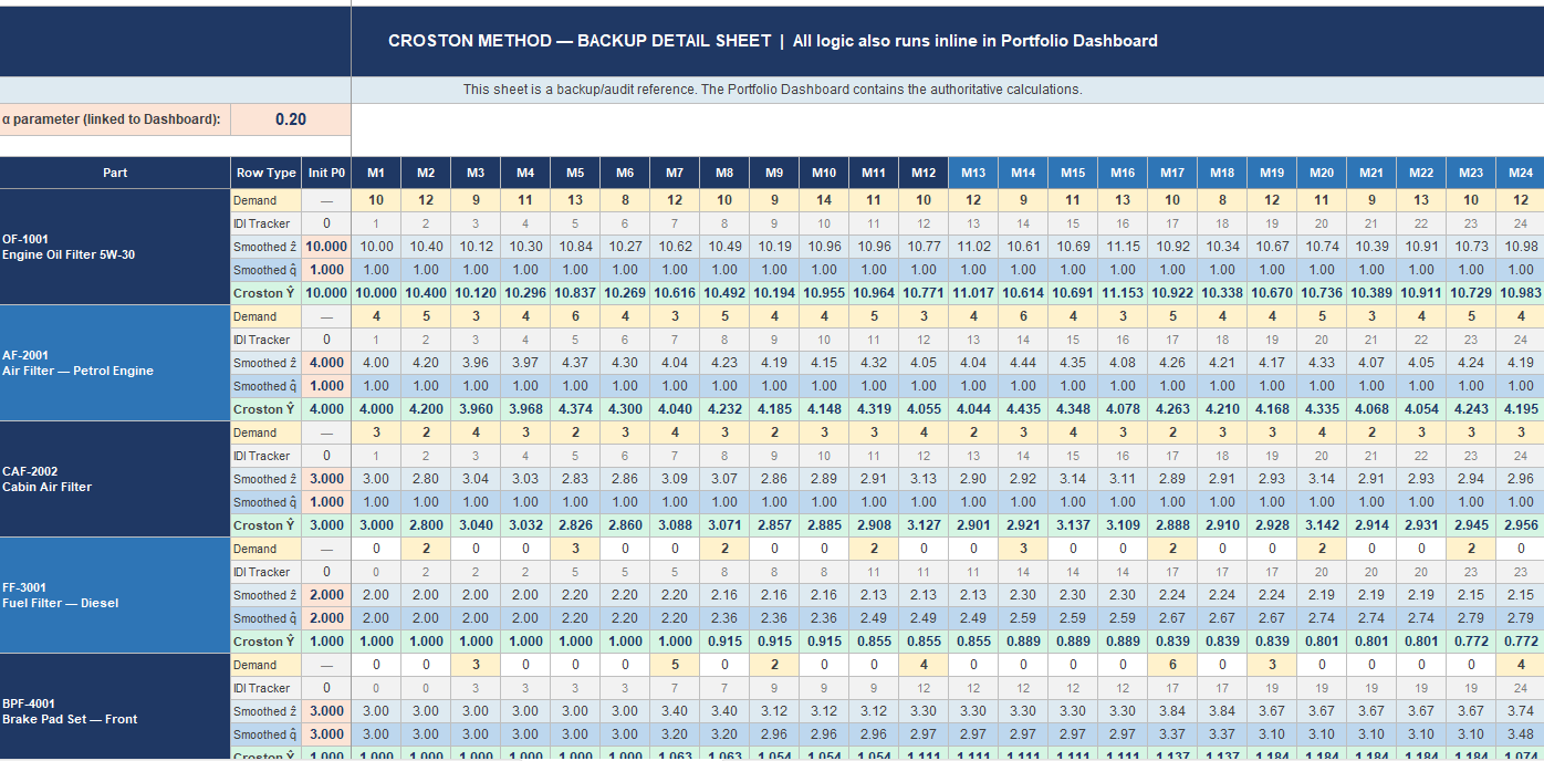
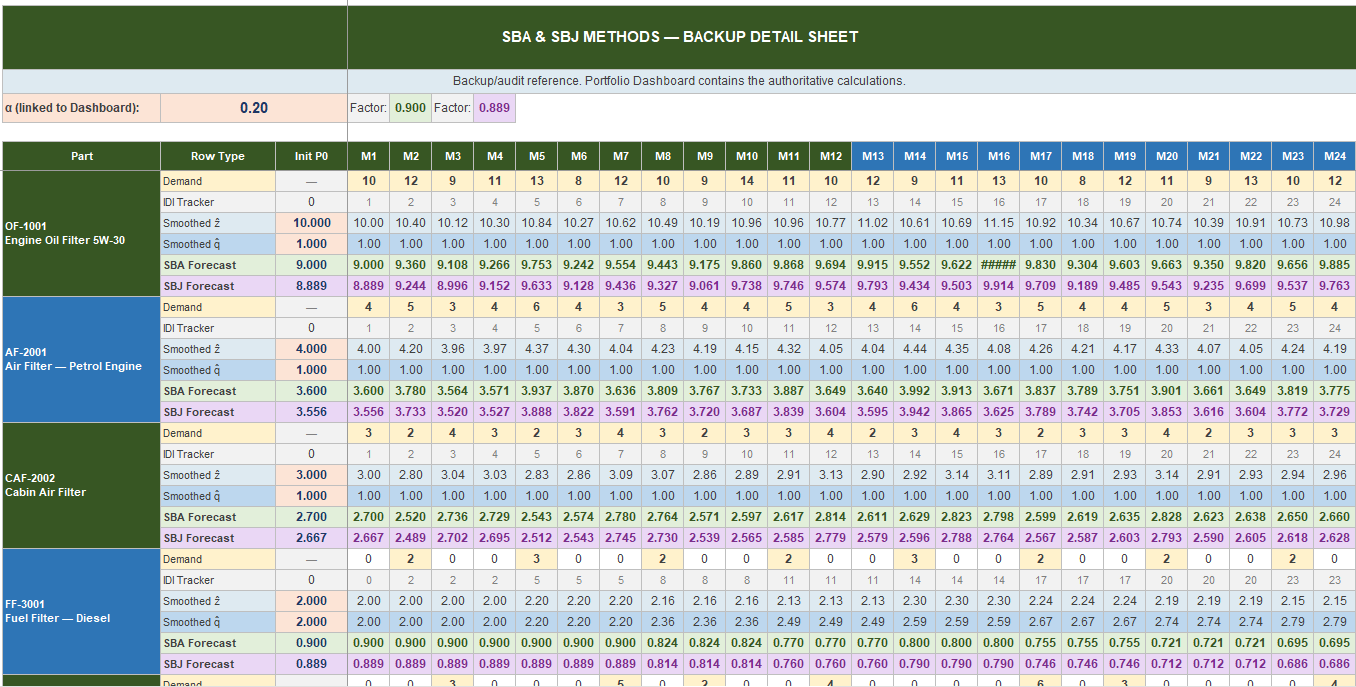
Eliminate the black-box problem by displaying every smoothing step. IDI Tracker, ẑ updates, q̂ updates, Croston ratio, SBA, and SBJ bias corrections are inline in the dashboard so analysts can trace every forecast figure back to the raw demand data.
4. Bridge the gap between forecast and inventory decision
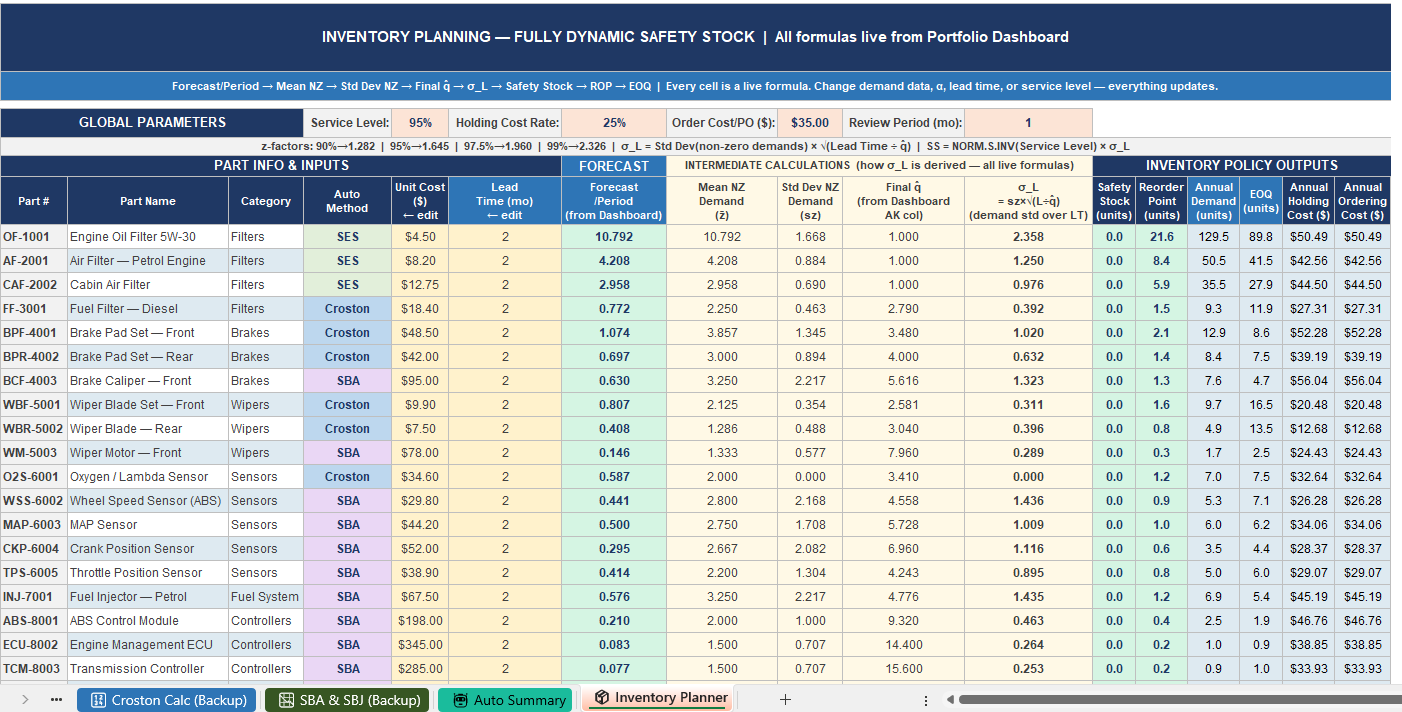
Connect the demand forecast directly to actionable inventory parameters: Safety Stock, Reorder Point, and EOQ, through a fully dynamic calculation chain where every variable is a live formula responding to changes in demand data, lead time, service level, and cost parameters.
5. Rehabilitate EOQ for spare parts environments
Demonstrate that EOQ is not inherently unsuitable for intermittent demand. The failure has always been the demand input, not the optimisation logic. With a principled forecast from Croston or SBA as the demand rate, EOQ produces defensible, actionable order quantities even for slow-moving SKUs.
6. Provide a scalable, production-ready portfolio template
Deliver a structured 20-SKU × 24-month working model that practitioners can immediately adapt to their own catalogue by replacing demand data with all formulas, classifications, and inventory outputs, updating automatically.
7. Build statistical literacy in the practitioner
Through visible intermediate calculations, colour-coded row labels, and a detailed companion chapter, develop the user's understanding of intermittent demand statistics — ρ, CV², exponential smoothing mechanics, bias correction, and sigma-based safety stock. Hence, the template becomes a learning instrument, not just a calculator.
Demand Pattern Conditions
This model is designed specifically for SKU catalogues where a significant proportion of items exhibit intermittent demand, meaning demand is absent in many periods and arrives sporadically when it does occur. It applies best when:
• At least 30–40% of SKUs in the catalogue have months with zero demand
• Demand arrives in irregular intervals rather than on a predictable cycle
• When demand does arrive, quantities vary — sometimes one unit, sometimes several
• The catalogue contains a mix of demand types within the same portfolio — some parts moving regularly, others rarely
If every SKU in the catalogue has positive demand in every period, standard exponential smoothing or moving average methods are sufficient, and this model is not necessary.
________________________________________
Industry and Application Conditions
This template is most directly applicable in:
• Automotive aftermarket and spare parts distribution — the primary use case for which the model was built, covering any spare part from filters, brake components, sensors, electrical assemblies, to controllers
• MRO (Maintenance, Repair, and Operations) inventory — industrial facilities managing replacement parts for machinery, equipment, and infrastructure
• Aviation parts and components — where demand is safety-critical, highly intermittent, and the cost of a stockout is disproportionate to the cost of holding
• Medical device and equipment spare parts — hospitals, clinics, and service organizations managing low-frequency, high-criticality replacement components
• Capital equipment manufacturers — managing after-sales service parts across a wide installed base with unpredictable failure rates
• Field service operations — technician van stock and regional warehouse replenishment, where demand is driven by unpredictable equipment failures
________________________________________
Inventory Management Conditions
The model delivers its greatest value when:
• The organization manages more than 50 active spare part SKUs, making manual classification impractical
• Lead times are meaningful, at least 1–3 months, making the Reorder Point calculation consequential
• Holding costs are significant enough that over-stocking carries a real financial penalty
• The organization currently uses a single forecasting method across all SKUs, regardless of their demand pattern
• Inventory decisions are currently driven by gut feel, fixed reorder quantities, or ERP defaults rather than data-driven safety stock and ROP calculations
________________________________________
Data Conditions
The model requires and works best with:
• A minimum of 12 months of demand history per SKU. 24 months is optimal for stable parameter estimation
• Demand recorded at monthly granularity. Weekly data can be aggregated, and daily data should be rolled up
• Demand figures representing actual customer orders or consumption, not replenishment orders or goods received quantities
• Reasonably clean data. Extreme one-off outliers (bulk fleet orders, data entry errors) should be investigated and treated before the model is run, as they will permanently inflate the smoothed ẑ estimate
________________________________________
Organizational Conditions
This best practice is most effective when:
• There is at least one analyst or planner with basic Excel competency to maintain and extend the model
• Management is willing to adopt a differentiated stocking policy, accepting that a cabin air filter and an ABS control module should be managed by fundamentally different rules
• The organization reviews its forecasting parameters at least annually, updating demand history, revisiting α, and checking for SKUs that have shifted classification zone
• There is a clear owner for inventory policy decisions, so the Safety Stock and ROP outputs from the model are translated into actual purchasing and stocking instructions
Conditions Where This Model Has Limitations
In the interest of transparency, this approach is less suitable when:
• Demand history is shorter than 12 months — insufficient observations for reliable smoothing parameter estimation
• The catalogue contains fewer than 10 SKUs — manual analysis is faster and equally accurate at that scale
• Demand is driven by known, scheduled events such as planned maintenance contracts or seasonal campaigns. In that case, causal or calendar-based forecasting models outperform statistical smoothing
• The organization operates in an environment where demand is so rare (fewer than 2 events in 24 months) that the entire catalogue sits in the rare/lumpy zone. At that point, expert judgement and criticality-based stocking policies dominate over any statistical forecast.