

Originally published: 04/11/2020 15:18
Publication number: ELQ-19862-1
View all versions & Certificate
Publication number: ELQ-19862-1
View all versions & Certificate

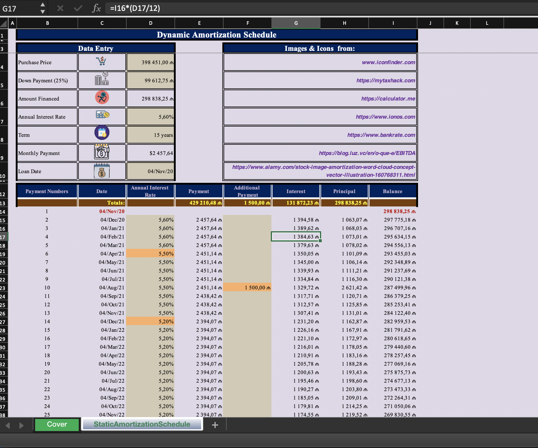
Dynamic Amortization Schedule
Dynamic Amortization Schedule in Microsoft Excel.
Further information
Financial Modelers are recommended to use this template
Two additional columns: Annual Interest Rate and Additional Payment differentiate make this template dynamic
Dynamic Array Functions would improve the quality of template